What changed in SQL Server 2012 regarding T-SQL - from the developers perspective

A very common need in application development is the use of data paging in SQL Server, so that only a limited amount of records are returned by queries, causing less data to be processed in the output and queries have a shorter response time. This scenario is quite common in applications, which tend to page data on the screen, both to avoid excess information and to reduce the time needed to load the information.

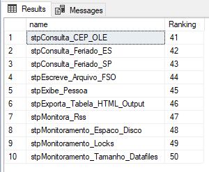
With the appearance of ROW_NUMBER() in SQL Server 2005, many people started using this function to create data pagination, working like this:

DECLARE
    @Pagina INT = 5,
    @ItensPorPagina INT = 10


SELECT *
FROM (
    SELECT [name], ROW_NUMBER() OVER(ORDER BY [name]) AS Ranking
    FROM sys.objects
) A
WHERE 
    A.Ranking >= ((@Pagina - 1) * @ItensPorPagina) + 1 
    AND A.Ranking < (@Pagina * @ItensPorPagina) + 1

Result:

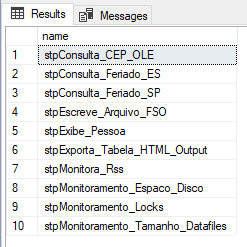
However, starting with SQL Server 2012, we have the native paging functionality in SQL Server itself, which many people end up not using due to lack of knowledge. We are talking about the OFFSET and FETCH feature, which work together to allow us to page our results before displaying and sending them to applications and clients.

See how it’s used, it’s simple:

SELECT [name]
FROM sys.objects
ORDER BY [name]
OFFSET 40 ROWS -- Linha de início: Vai começar a retornar a partir da linha 40
  FETCH NEXT 10 ROWS ONLY -- Quantidade de linhas para retornar: Vai retornar as próximas 10 linhas

Result:

If you want to know more about this feature, be sure to visit my article SQL Server – How to create data pagination in the results of a query with OFFSET and FETCH

An old acquaintance of Oracle DBA's, the Sequence feature was introduced in SQL Server 2012 and consists of creating sequences (similar to IDENTITY) not associated with a specific object, that is, you can create a sequence for a specific table or you can use a sequence for more than one table so that the ID numbers will not be repeated between the tables involved.

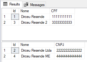
Classic example: Pessoa_Fisica and Pessoa_Juridica tables. If you use IDENTITY to generate a sequential, the 2 tables will have a record with ID = 25, for example. If you use a single sequence to control the ID of these two tables, the ID = 25 will only exist in one of the two tables, working like this:

Test source code

CREATE SEQUENCE dbo.[seq_Pessoa]
AS [INT]
    START WITH 1
    INCREMENT BY 1
    MINVALUE 1
    MAXVALUE 999999999
    CYCLE
    CACHE
GO

CREATE TABLE dbo.Pessoa_Fisica (
    Id INT DEFAULT NEXT VALUE FOR dbo.seq_Pessoa,
    Nome VARCHAR(100),
    CPF VARCHAR(11)
)

CREATE TABLE dbo.Pessoa_Juridica (
    Id INT DEFAULT NEXT VALUE FOR dbo.seq_Pessoa,
    Nome VARCHAR(100),
    CNPJ VARCHAR(14)
)

INSERT INTO dbo.Pessoa_Fisica (Nome, CPF)
VALUES('Dirceu Resende', '11111111111')

INSERT INTO dbo.Pessoa_Juridica (Nome, CNPJ)
VALUES('Dirceu Resende Ltda', '22222222222222')

INSERT INTO dbo.Pessoa_Fisica (Nome, CPF)
VALUES('Dirceu Resende 2', '33333333333')

INSERT INTO dbo.Pessoa_Juridica (Nome, CNPJ)
VALUES('Dirceu Resende ME', '44444444444444')

SELECT * FROM dbo.Pessoa_Fisica
SELECT * FROM dbo.Pessoa_Juridica

Result

If you want to know more about Sequences in SQL Server, read my article SQL Server 2012 – Working with Sequences and comparisons with IDENTITY.

Every good developer of queries and database routines uses error and exception handling in their T-SQL codes. Starting with SQL Server 2005, Microsoft introduced the TRY…CATCH feature in T-SQL, where we could generate exceptions using the command RAISEERROR. As of SQL Server 2012, the new method of THROW, which allows you to simplify and make the generation of exceptions in the database more intelligent.

Treatment of division by zero using RAISEERROR

BEGIN TRY
    SELECT 1/0
END TRY

BEGIN CATCH
    
    DECLARE 
        @MsgErro VARCHAR(MAX) = ERROR_MESSAGE(),
        @IntState INT = ERROR_STATE(),
        @IntSeverity INT = ERROR_SEVERITY()

    RAISERROR(@MsgErro, @IntSeverity, @IntState) WITH NOWAIT

END CATCH

Result:

Treatment of division by zero using THROW

BEGIN TRY
    SELECT 1/0
END TRY

BEGIN CATCH
    THROW
END CATCH

Result:

Much simpler, right? And it doesn't stop there... To use personalized messages, THROW is also much simpler, as the message error code (error_number) does not need to be registered in sys.messages.

Another advantage of THROW is that it is possible to record the output of error messages returned by THROW in a history table (using RAISEERROR you cannot capture the return of the command, but you can also create this history by inserting the records in the table and capturing the messages using the ERROR_% functions, such as ERROR_MESSAGE())

To learn more about the advantages of THROW, be sure to check out the article Applying error handling in Microsoft SQL Server 2012 and 2014 – using the throw command.

Well known by programmers, the IIF function was introduced in SQL Server 2012 and its objective is to simplify simple logical operations, which have only 2 possible results.

Simple example with CASE

SELECT (CASE WHEN DATEPART(HOUR, GETDATE()) < 12 THEN 'AM' ELSE 'PM' END)

Simple example with IIF

SELECT IIF(DATEPART(HOUR, GETDATE()) < 12, 'AM', 'PM')

Much simpler, right? However, if you need several results, I recommend continuing to use CASE, as the IIF ends up becoming very complex to maintain when it is nested with several other IIFs.

Another function available starting in SQL Server 2012 is the CHOOSE logic function. This function allows you to retrieve a value based on the numerical position (index) of a list of values. This function can be used to simplify some scenarios in which you would have to place several CASE conditions.

Usage example:

SELECT CHOOSE(5, 
    'Janeiro', 
    'Fevereiro', 
    'Março', 
    'Abril', 
    'Maio', 
    'Junho', 
    'Julho', 
    'Agosto', 
    'Setembro', 
    'Novembro', 
    'Dezembro'
)

Result:

Another example, now retrieving the index from the result of a function:

SELECT 
    GETDATE() AS Hoje,
    DATEPART(WEEKDAY, GETDATE()) AS Dia_Semana,
    CHOOSE(DATEPART(WEEKDAY, GETDATE()), 
        'Domingo',
        'Segunda-feira',
        'Terça-feira',
        'Quarta-feira',
        'Quinta-feira',
        'Sexta-feira',
        'Sábado'
    ) AS Nome_Dia_Semana

Result:

Examples using indexes outside the list and indexes with decimals

SELECT 
    CHOOSE(-1, 
        'Domingo',
        'Segunda-feira',
        'Terça-feira',
        'Quarta-feira',
        'Quinta-feira',
        'Sexta-feira',
        'Sábado'
    ) AS Nome_Dia_Semana1,
    CHOOSE(4.9, 
        'Domingo',
        'Segunda-feira',
        'Terça-feira',
        'Quarta-feira',
        'Quinta-feira',
        'Sexta-feira',
        'Sábado'
    ) AS Nome_Dia_Semana2

Result:

As we can see above, when the index of the CHOOSE function is not in the list range, the function will return NULL. And when we use an index with decimal places, the index will be converted (truncated) to an integer.

Note: Internally, CHOOSE is a shortcut for CASE, so the 2 have the same performance.

Functions widely used in the daily lives of Query developers, the data type conversion functions underwent a major evolution in SQL Server 2012 with the new functions PARSE, TRY_PARSE, TRY_CONVERT and TRY_CAST.

The function PARISH (available for dates and numbers) is very useful for converting some formats other than the standard, which CAST and CONVERT cannot convert, like the example below:

SELECT CAST('Sábado, 29 de dezembro de 2018' AS DATETIME) AS [Cast] -- Erro
GO

SELECT CONVERT(DATETIME, 'Sábado, 29 de dezembro de 2018') AS [CONVERT] -- Erro
GO

SELECT PARSE('Sábado, 29 de dezembro de 2018' AS DATETIME USING 'pt-BR') AS [PARSE] -- Sucesso
GO

Result:

As an evolution of the PARSE function, we have the function TRY_PARSE, which has basically the same behavior as the PARSE function, but with the difference that when conversion is not possible, instead of returning an exception during processing, it will just return NULL.

Example:

-- Nesse exemplo, será gerada uma exceção durante a execução do código T-SQL
-- Msg 9819, Level 16, State 1, Line 1: Error converting string value 'Domingo, 29 de dezembro de 2018' into data type datetime using culture 'pt-BR'.
SELECT PARSE('Domingo, 29 de dezembro de 2018' AS DATETIME USING 'pt-BR') AS [PARSE]
GO

-- Aqui vai apenas retornar NULL
SELECT TRY_PARSE('Domingo, 29 de dezembro de 2018' AS DATETIME USING 'pt-BR') AS [PARSE]
GO

The same thing happens with functions TRY_CONVERT and TRY_CAST, which have the same behavior as the original functions, but do not generate an exception when unable to perform a conversion.

Usage examples:

-- Sucesso (2018-12-28 00:00:00.000)
SELECT CAST('2018-12-28' AS DATETIME)
GO

-- Erro: The conversion of a varchar data type to a datetime data type resulted in an out-of-range value.
SELECT CAST('2018-12-99' AS DATETIME)
GO

-- NULL
SELECT TRY_CAST('2018-12-99' AS DATETIME)
GO

-- Sucesso (2018-12-28 00:00:00.000)
SELECT CONVERT(DATETIME, '2018-12-28')
GO

-- Erro: The conversion of a varchar data type to a datetime data type resulted in an out-of-range value.
SELECT CONVERT(DATETIME, '2018-12-99')
GO

-- NULL
SELECT TRY_CONVERT(DATETIME, '2018-12-99')
GO

Result:

To learn more about data processing and conversions, see my article SQL Server – How to identify data conversion errors using TRY_CAST, TRY_CONVERT, TRY_PARSE, ISNUMERIC and ISDATE.

Very interesting function for those who work with BI and calculations involving dates and the end of the month. Basically, this function returns the last day of the month of the given date.

Usage examples

SELECT 
    EOMONTH('2018-01-01') AS Janeiro,
    EOMONTH('2018-02-12') AS Fevereiro,
    EOMONTH('2018-03-15') AS [Março],
    EOMONTH('2018-04-17') AS Abril,
    EOMONTH('2018-05-29') AS Maio,
    EOMONTH('2018-06-05') AS Junho,
    EOMONTH('2018-07-04') AS Julho,
    EOMONTH('2018-08-24') AS Agosto,
    EOMONTH('2018-09-21') AS Setembro,
    EOMONTH('2018-10-11') AS Outubro,
    EOMONTH('2018-11-10') AS Novembro,
    EOMONTH('2018-12-03') AS Dezembro

Result

As of SQL Server 2012, we have 6 new functions for generating dates from integers, which was quite annoying to do in previous versions of SQL Server:

• DATEFROMPARTS ( year, month, day)
• DATETIME2FROMPARTS ( year, month, day, hour, minute, seconds, fractions, precision )
• DATETIMEFROMPARTS ( year, month, day, hour, minute, seconds, milliseconds )
• DATETIMEOFFSETFROMPARTS ( year, month, day, hour, minute, seconds, fractions, hour_offset, minute_offset, precision )
• SMALLDATETIMEFROMPARTS ( year, month, day, hour, minute )
• TIMEFROMPARTS ( hour, minute, seconds, fractions, precision )

Script for generating test data:

IF (OBJECT_ID('tempdb..#Dados') IS NOT NULL) DROP TABLE #Dados
CREATE TABLE #Dados (
    Ano INT,
    Mes INT,
    Dia INT,
    Hora INT,
    Minuto INT,
    Segundo INT,
    Millisegundo INT,
    Offset_Hora INT,
    Offset_Minuto INT
)

INSERT INTO #Dados
VALUES
    (2018, 12, 19, 14, 39, 1, 123, 3, 30),
    (1987, 5, 28, 21, 22, 59, 999, 3, 0),
    (2018, 12, 31, 23, 59, 59, 999, 0, 0)

Example of the DATEFROMPARTS function and how we did it before SQL Server 2012:

-- Antes do SQL Server 2012: Utilizando CAST/CONVERT
SELECT
    CAST(CAST(Ano AS VARCHAR(4)) + '-' + CAST(Mes AS VARCHAR(2)) + '-' + CAST(Dia AS VARCHAR(2)) AS DATE) AS [CAST_DATE]
FROM
    #Dados

-- A partir do SQL Server 2012: DATEFROMPARTS
SELECT 
    DATEFROMPARTS (Ano, Mes, Dia) AS [DATEFROMPARTS]
FROM
    #Dados

Result:

Example using the 6 functions together

SELECT 
    DATEFROMPARTS (Ano, Mes, Dia) AS [DATEFROMPARTS],
    DATETIME2FROMPARTS (Ano, Mes, Dia, Hora, Minuto, Segundo, Millisegundo, 7) AS [DATETIME2FROMPARTS],
    DATETIMEFROMPARTS (Ano, Mes, Dia, Hora, Minuto, Segundo, Millisegundo) AS [DATETIMEFROMPARTS],
    DATETIMEOFFSETFROMPARTS (Ano, Mes, Dia, Hora, Minuto, Segundo, Millisegundo, Offset_Hora, Offset_Minuto, 7) AS [DATETIMEOFFSETFROMPARTS],
    SMALLDATETIMEFROMPARTS (Ano, Mes, Dia, Hora, Minuto) AS [SMALLDATETIMEFROMPARTS],
    TIMEFROMPARTS (Hora, Minuto, Segundo, Millisegundo, 7) AS [TIMEFROMPARTS]
FROM
    #Dados

Result:

One of the most useful functions in the daily lives of those who work creating queries and BI routines, the function FORMAT allows you to apply custom masks to dates and numbers, very similar to the C# string.ToString() method.

Some examples of the use of FORMAT – Numbers

SELECT
    FORMAT(123456.99, 'C'), -- Formato de moeda padrão
    FORMAT(-123456.987654321, 'C4'), -- Formato de moeda com 4 casas decimais
    FORMAT(123456.987654321, 'C2', 'pt-br') -- Formato de moeda forçando a localidade pra Brasil e 2 casas decimais

SELECT
    FORMAT(123456.99, 'D'), -- Formato de número inteiro com valores numeric (NULL)
    FORMAT(123456, 'D'), -- Formato de número inteiro
    FORMAT(-123456, 'D4'), -- Formato de número inteiro com valores negativos
    FORMAT(123456, 'D10', 'pt-br'), -- formato de número inteiro com tamanho fixo em 10 caracteres
    FORMAT(-123456, 'D10', 'pt-br') -- formato de número inteiro com tamanho fixo em 10 caracteres

SELECT
    FORMAT(123456.99, 'E'), -- Formato de notação científica
    FORMAT(123456.99, 'E4') -- Formato de notação científica e 4 casas decimais de precisão

SELECT
    FORMAT(1, 'P'), -- Formato de porcentagem
    FORMAT(1, 'P2'), -- Formato de porcentagem com 2 casas decimais
    FORMAT(0.91, 'P'), -- Formato de porcentagem
    FORMAT(0.005, 'P4') -- Formato de porcentagem com 4 casas decimais

SELECT
    FORMAT(255, 'X'), -- Formato hexadecimal
    FORMAT(512, 'X8') -- Formato hexadecimal fixando o retorno em 8 caracteres

Result

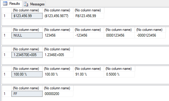
Other examples with numbers:

SELECT
    -- Formato de moeda brasileira (manualmente)
    FORMAT(123456789.9, 'R$ ###,###,###,###.00'),
    -- Utilizando sessão (;) para formatar valores positivos e negativos
    FORMAT(123456789.9, 'R$ ###,###,###,###.00;-R$ ###,###,###,###.00'), 
    
    -- Utilizando sessão (;) para formatar valores positivos e negativos
    FORMAT(-123456789.9, 'R$ ###,###,###,###.00;-R$ ###,###,###,###.00'), 
    -- Utilizando sessão (;) para formatar valores positivos e negativos
    FORMAT(-123456789.9, 'R$ ###,###,###,###.00;(R$ ###,###,###,###.00)'),
    
    -- Formatando porcentagem com 2 casas decimais
    FORMAT(0.9975, '#.00%'), 
    -- Formatando porcentagem com 4 casas decimais
    FORMAT(0.997521654, '#.0000%'),
    -- Formatando porcentagem com 4 casas decimais
    FORMAT(123456789.997521654, '#.0000%'),
    
    -- Formatando porcentagem com 2 casas decimais e utilizando sessão (;)
    FORMAT(0.123456789, '#.00%;-#.00%'),
    -- Formatando porcentagem com 2 casas decimais e utilizando sessão (;)
    FORMAT(-0.123456789, '#.00%;-#.00%'),
    -- Formatando porcentagem com 2 casas decimais e utilizando sessão (;)
    FORMAT(-0.123456789, '#.00%;(#.00%)')

Result:

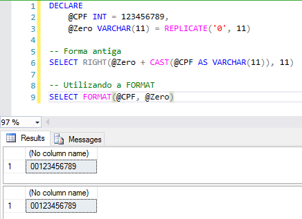
Filling number with leading zeros:

Some examples of the use of FORMAT – Dates

SET LANGUAGE 'English'

SELECT
    FORMAT(GETDATE(), 'd'), -- Padrão de data abreviada.
    FORMAT(GETDATE(), 'D'), -- Padrão de data completa.

    FORMAT(GETDATE(), 'R'), -- Padrão RFC1123

    FORMAT(GETDATE(), 't'), -- Padrão de hora abreviada.
    FORMAT(GETDATE(), 'T') -- Padrão de hora completa.
    

SET LANGUAGE 'Brazilian'

SELECT
    FORMAT(GETDATE(), 'd'), -- Padrão de data abreviada.
    FORMAT(GETDATE(), 'D'), -- Padrão de data completa.

    FORMAT(GETDATE(), 'R'), -- Padrão RFC1123

    FORMAT(GETDATE(), 't'), -- Padrão de hora abreviada.
    FORMAT(GETDATE(), 'T') -- Padrão de hora completa.

Result:

Custom Date Formatting:

SELECT
    -- Formato de data típico do Brasil
    FORMAT(GETDATE(), 'dd/MM/yyyy'),

    -- Formato de data/hora típico dos EUA
    FORMAT(GETDATE(), 'yyyy-MM-dd HH:mm:ss.fff'),

    -- Exibindo a data por extenso
    FORMAT(GETDATE(), 'dddd, dd \d\e MMMM \d\e yyyy'),

    -- Exibindo a data por extenso (forçando o idioma pra PT-BR)
    FORMAT(GETDATE(), 'dddd, dd \d\e MMMM \d\e yyyy', 'pt-br'),

    -- Exibindo a data/hora, mas zerando os minutos e segundos
    FORMAT(GETDATE(), 'dd/MM/yyyy HH:00:00', 'pt-br')

Result:

If you want to know more about the FORMAT function, read my article SQL Server – Using the FORMAT function to apply masks and formatting to numbers and dates.

Available starting with SQL Server 2012, the function CONCAT allows you to concatenate variables, strings and/or columns in a more practical way, which I will demonstrate its advantages below:

Generating data for examples

IF (OBJECT_ID('tempdb..#Dados') IS NOT NULL) DROP TABLE #Dados
CREATE TABLE #Dados (
    Dt_Nascimento DATE,
    Nome1 VARCHAR(50),
    Nome2 VARCHAR(50),
    Idade AS CONVERT(INT, (DATEDIFF(DAY, Dt_Nascimento, GETDATE()) / 365.25))
)

INSERT INTO #Dados
VALUES
    ('1987-05-28', 'Dirceu', 'Resende'),
    ('1987-01-15', 'Patricia', 'Resende'),
    ('1987-01-15', 'Teste', NULL)

Examples

-- Antes do SQL Server 2012: Utilizando CAST/CONVERT
SELECT
    Nome1 + ' ' + Nome2 + ' | ' + CAST(Idade AS VARCHAR(3)) + ' | ' + CAST(Dt_Nascimento AS VARCHAR(40)) AS [Antes do SQL Server 2012]
FROM
    #Dados

-- A partir do SQL Server 2012: Utilizando CONCAT
SELECT
    CONCAT(Nome1, ' ', Nome2, ' | ', Idade, ' | ', Dt_Nascimento) AS [A partir do SQL Server 2012]
FROM
    #Dados

Result:

As you can see, the CONCAT function automatically converts data types to varchar and also handles NULL values ​​and converts them to empty strings. In other words, CONCAT is simpler, but what about performance? How is it?

At least in the tests I did, CONCAT proved to be faster than traditional concatenation (using “+”). Simpler and faster.

Very interesting analytical functions, the function FIRST_VALUE returns the first value of a resultset, where you can define an optional break (PARTITION BY) and a rule to order the results (ORDER BY). Now the function LAST_VALUE, does the opposite, returning the last value from this data set.

T-SQL script for creating data for the example:

IF (OBJECT_ID('tempdb..#Dados') IS NOT NULL) DROP TABLE #Dados
CREATE TABLE #Dados (
    Id INT IDENTITY(1,1),
    Nome VARCHAR(50),
    Idade INT
)

INSERT INTO #Dados
VALUES
    ('Dirceu Resende', 31),
    ('Joãozinho das Naves', 33),
    ('Rafael Sudré', 48),
    ('Potássio', 27),
    ('Rafaela', 25),
    ('Jodinei', 39)

Example 1 – Identifying the oldest and youngest ages and the names of these people

-- Antes do SQL Server 2012: MIN/MAX e Subquery
SELECT
    *,
    (SELECT MIN(Idade) FROM #Dados) AS Menor_Idade,
    (SELECT MAX(Idade) FROM #Dados) AS Maior_Idade,
    (SELECT TOP(1) Nome FROM #Dados ORDER BY Idade) AS Nome_Menor_Idade,
    (SELECT TOP(1) Nome FROM #Dados ORDER BY Idade DESC) AS Nome_Maior_Idade
FROM
    #Dados


-- A partir do SQL Server 2012: FIRST_VALUE
SELECT
    *,
    FIRST_VALUE(Idade) OVER(ORDER BY Idade) AS Menor_Idade,
    FIRST_VALUE(Idade) OVER(ORDER BY Idade DESC) AS Maior_Idade,
    FIRST_VALUE(Nome) OVER(ORDER BY Idade) AS Nome_Menor_Idade,
    FIRST_VALUE(Nome) OVER(ORDER BY Idade DESC) AS Nome_Maior_Idade
FROM
    #Dados

Result:

Well, the code is much simpler and cleaner. Speaking of performance, there are several ways to achieve this goal, with more performant queries than the one I used in the first example, but I wanted to make the code as simple as possible. If you actually use this type of programming in your code, it's a good idea to review your queries, as they have very poor performance.

See what the execution plan looks like for the first query and the query using the FIRST_VALUE function:

And now let's use the LAST_VALUE function to return the largest records in the dataset:

SELECT
    *,
    FIRST_VALUE(Idade) OVER(ORDER BY Idade) AS Menor_Idade,
    LAST_VALUE(Idade) OVER(ORDER BY Idade) AS Maior_Idade,
    FIRST_VALUE(Nome) OVER(ORDER BY Idade) AS Nome_Menor_Idade,
    LAST_VALUE(Nome) OVER(ORDER BY Idade) AS Nome_Maior_Idade
FROM
    #Dados

Result:

Huh.. The LAST_VALUE function did not bring the last value but the value of the current line.. This happens due to the concept of frame. The frame allows you to specify a set of rows for the “window”, which is even smaller than the partition. The default frame contains lines starting with the first line and up to the current line. For line 1, the “window” is just line 1. For line 3, the window contains lines 1 through 3. When using FIRST_VALUE, the first line is included by default, so you don't have to worry about it to get the results you expect.

For the LAST_VALUE function to actually return the last value of the entire data set, we will use the ROWS BETWEEN CURRENT ROW AND UNBOUNDED FOLLOWING parameters together with the LAST_VALUE function, which causes the window to start from the current line to the last line of the partition.

New script using the LAST_VALUE function:

SELECT
    *,
    FIRST_VALUE(Idade) OVER(ORDER BY Idade) AS Menor_Idade,
    LAST_VALUE(Idade) OVER(ORDER BY Idade ROWS BETWEEN CURRENT ROW AND UNBOUNDED FOLLOWING) AS Maior_Idade,
    FIRST_VALUE(Nome) OVER(ORDER BY Idade) AS Nome_Menor_Idade,
    LAST_VALUE(Nome) OVER(ORDER BY Idade ROWS BETWEEN CURRENT ROW AND UNBOUNDED FOLLOWING) AS Nome_Maior_Idade
FROM
    #Dados

Result:

Starting with SQL Server 2012, we have two more analytical functions available to access the record before a record (LAG) and subsequent registration (LEAD).

T-SQL script to generate the test data:

IF (OBJECT_ID('tempdb..#Dados') IS NOT NULL) DROP TABLE #Dados
CREATE TABLE #Dados (
    Id INT IDENTITY(1,1),
    Nome VARCHAR(50),
    Idade INT
)

INSERT INTO #Dados
VALUES
    ('Dirceu Resende', 31),
    ('Joãozinho das Naves', 33),
    ('Rafael Sudré', 48),
    ('Potássio', 27),
    ('Rafaela', 25),
    ('Jodinei', 39)

Imagine that I want to create a pointer and access who is the next ID and the previous ID of the current record. Before SQL Server 2008, we would need to create self-joins to complete this task. Starting with SQL Server 2012, we can use the LAG and LEAD functions for this need:

-- Antes do SQL Server 2008: Self-Joins
SELECT 
    A.*,
    B.Id AS Id_Proximo,
    C.Id AS Id_Anterior
FROM
    #Dados A
    LEFT JOIN #Dados B ON B.Id = A.Id + 1
    LEFT JOIN #Dados C ON C.Id = A.Id - 1


-- A partir do SQL Server 2012: LAG e LEAD
SELECT 
    A.*,
    LEAD(Id) OVER(ORDER BY Id) AS Id_Proximo,
    LAG(Id) OVER(ORDER BY Id) AS Id_Anterior
FROM
    #Dados A

Result:

Much simpler and cleaner code. Let's analyze the performance of the two queries now:

Yes, although LAG and LEAD are much simpler and more readable, their performance ends up being a little lower than Self-Joins, probably due to the ordering that is done to apply the functions. I'm going to insert a larger volume of records (3 million records) to check if the performance is still worse than Self-Joins, which I believe doesn't make sense, since Self-Join performs several readings on the table and functions, in theory, should only do 1.

Test results with 3 million records (surprised me):

Execution plan with SELF-JOIN:

Execution plan with LED and LEAD:

I imagined that by having a simpler plan and making fewer readings from the table, the functions would have a much better performance than self-joins, but because of a very heavy SORT operator, the performance using the functions ended up being worse, as we can see in the execution plan and the warning for the sort operator:

In short, if you are working with small data sets, you can use the LAG and LEAD functions without any problems, as the code is more readable. If you need to use this on large volumes of data, test the self-join to evaluate how the performance will be in your scenario.

A scenario that is somewhat common in the daily lives of data professionals, capturing data returned by Stored Procedures can end up being a bit of work when it is necessary to perform data type conversions. In this case, it is necessary to use an intermediate table to perform the data conversion and then use the necessary data.

As of SQL Server 2012, we can now use the WITH RESULT SETS clause when executing Stored Procedures, so that we can change the name and type of fields returned by Stored Procedures, in a very simple and practical way.

Example 1:

CREATE PROCEDURE dbo.stpLista_Tabelas
AS
BEGIN
    
    SELECT 
        [object_id],
        [name],
        [type_desc],
        create_date
    FROM 
        sys.tables

END


-- Executa a Stored Procedure
EXEC dbo.stpLista_Tabelas
GO

EXEC dbo.stpLista_Tabelas
WITH RESULT SETS ((
    [id_tabela] int,
    [nome_tabela] varchar(100),
    [tipo] varchar(50),
    [data_criacao] date
))

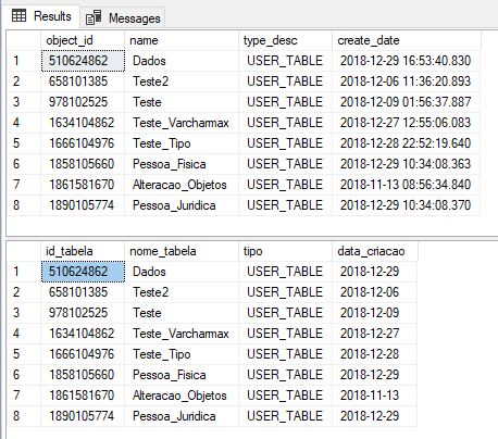
Result:

If the Stored Procedure returns more than one set of data, you can use the WITH RESULT SETS clause like this:

CREATE PROCEDURE dbo.stpLista_Tabelas2
AS
BEGIN
    
    SELECT 
        [object_id],
        [name],
        [type_desc],
        create_date
    FROM 
        sys.tables


    SELECT 
        [object_id],
        [name],
        [type_desc],
        create_date
    FROM 
        sys.objects

END


-- Executa a Stored Procedure
EXEC dbo.stpLista_Tabelas2
GO

EXEC dbo.stpLista_Tabelas2
WITH RESULT SETS (
    (
        [id_tabela] int,
        [nome_tabela] varchar(100),
        [tipo] varchar(50),
        [data_criacao] date
    ),
    (
        [id_objeto] int,
        [nome_objeto] varchar(100),
        [tipo] varchar(50),
        [data_criacao] date
    )
)

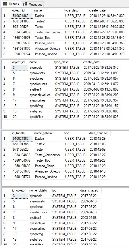
Result:

A new feature that was added to SQL Server 2012 is the possibility of returning x% of data from a table, using the TOP command. This is very useful when you want to return a measured sample of data in percentage form.

Its use is practically the same as the traditional and already known TOP:

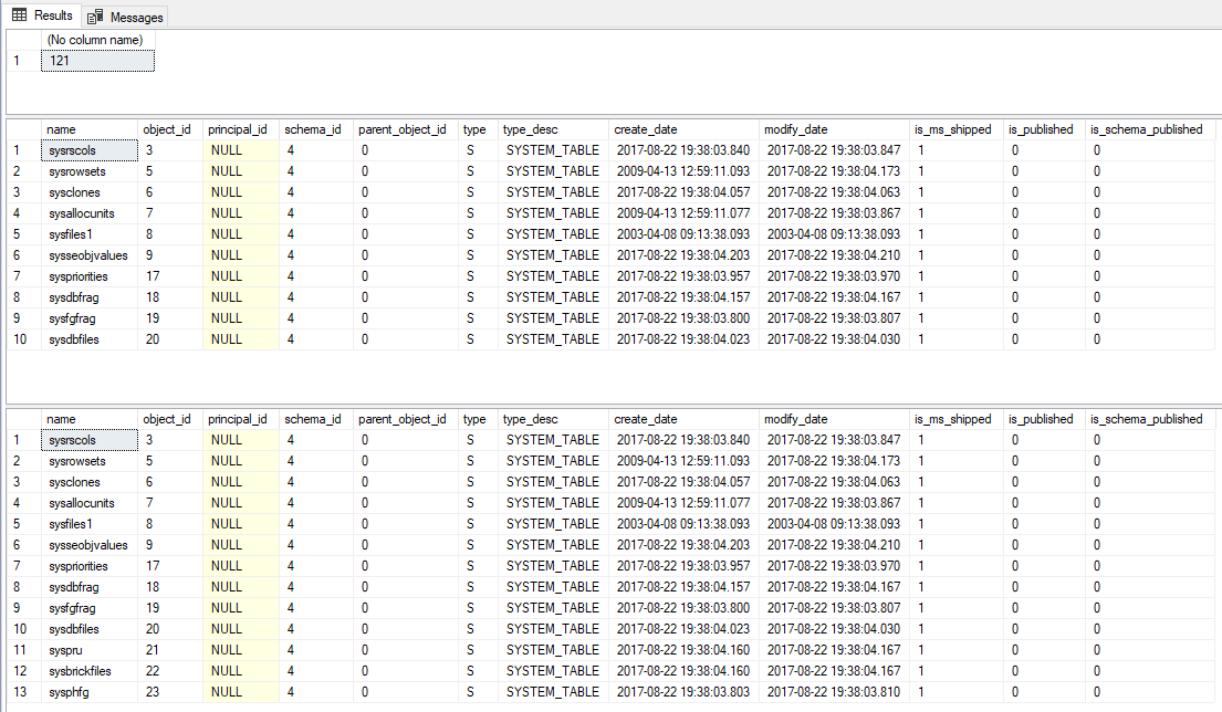
-- Conta quantos objetos existem na sys.objects (121)
SELECT COUNT(*) FROM sys.objects

-- Retorna 10 linhas da view sys.objects
SELECT TOP 10 * FROM sys.objects

-- Retorna 10% das linhas da view sys.objects (arredondando para cima - CEILING)
SELECT TOP 10 PERCENT * FROM sys.objects

Result:

Until version 2008, SQL Server had 2 functions for calculations with logarithms: LOG (standard base) and LOG10. If you needed to use a personalized basis in your mathematical calculations, you would have to implement the calculation manually.

Starting with SQL Server 2012, the LOG function now has a second optional parameter, where you can inform which base you want to use in your logarithm calculation:
Example:

SELECT LOG(256, 4) / LOG(2, 22);