Hey guys,
Good morning!
In this post I will talk about a subject that is nothing new in SQL Server, it has been present since SQL Server 2008, but I don't see many people using it in their queries, which is data grouping (summarization) using ROLLUP, CUBE and GROUPING SETS.
This type of resource is especially useful for generating totals and subtotals without having to create multiple subqueries, as it allows you to perform this task in a single command, as I will demonstrate below.
To create an AutoSum feature in your dataset, just like Excel implements it, see more in the post SQL Server – How to create an AutoSum (same as Excel) using Window functions
Test Base
For the examples in this post, I will provide the base below so that we can create a testing and demonstration environment.
IF (OBJECT_ID('tempdb..#Produtos') IS NOT NULL) DROP TABLE #Produtos
CREATE TABLE #Produtos (
    Codigo INT IDENTITY(1, 1) NOT NULL PRIMARY KEY,
    Ds_Produto VARCHAR(50) NOT NULL,
    Ds_Categoria VARCHAR(50) NOT NULL,
    Preco NUMERIC(18, 2) NOT NULL
)

IF (OBJECT_ID('tempdb..#Vendas') IS NOT NULL) DROP TABLE #Vendas
CREATE TABLE #Vendas (
    Codigo INT IDENTITY(1, 1) NOT NULL PRIMARY KEY,
    Dt_Venda DATETIME NOT NULL,
    Cd_Produto INT NOT NULL
)


INSERT INTO #Produtos ( Ds_Produto, Ds_Categoria, Preco )
VALUES
    ( 'Processador i7', 'Informática', 1500.00 ),
    ( 'Processador i5', 'Informática', 1000.00 ),
    ( 'Processador i3', 'Informática', 500.00 ),
    ( 'Placa de Vídeo Nvidia', 'Informática', 2000.00 ),
    ( 'Placa de Vídeo Radeon', 'Informática', 1500.00 ),
    ( 'Celular Apple', 'Celulares', 10000.00 ),
    ( 'Celular Samsung', 'Celulares', 2500.00 ),
    ( 'Celular Sony', 'Celulares', 4200.00 ),
    ( 'Celular LG', 'Celulares', 1000.00 ),
    ( 'Cama', 'Utilidades do Lar', 2000.00 ),
    ( 'Toalha', 'Utilidades do Lar', 40.00 ),
    ( 'Lençol', 'Utilidades do Lar', 60.00 ),
    ( 'Cadeira', 'Utilidades do Lar', 200.00 ),
    ( 'Mesa', 'Utilidades do Lar', 1000.00 ),
    ( 'Talheres', 'Utilidades do Lar', 50.00 )


DECLARE @Contador INT = 1, @Total INT = 100

WHILE(@Contador <= @Total)
BEGIN

    INSERT INTO #Vendas ( Cd_Produto, Dt_Venda )
    SELECT
        (SELECT TOP 1 Codigo FROM #Produtos ORDER BY NEWID()) AS Cd_Produto,
        DATEADD(DAY, (CAST(RAND() * 364 AS INT)), '2017-01-01') AS Dt_Venda

    SET @Contador += 1

END
In a simple data grouping, just bringing the quantities filtering by category and product, we were able to return this view using the query below:
SELECT
    B.Ds_Categoria,
    B.Ds_Produto,
    COUNT(*) AS Qt_Vendas,
    SUM(B.Preco) AS Vl_Total
FROM
    #Vendas A
    JOIN #Produtos B ON A.Cd_Produto = B.Codigo
GROUP BY
    B.Ds_Categoria,
    B.Ds_Produto
ORDER BY
    1, 2
Summarizing the values
But what if you need to group the data creating a totalizer for each category and at the end a general totalizer? How would you do it?
Using UNION ALL
A traditional way of meeting this need is using subquery with UNION ALL, so that you return 3 resultsets containing the analytical data, the totalizers by category and then the general sum. The greater the number of filters, the more complex your subquery will be, as it will need more queries at each level.
SELECT
    *
FROM (

    SELECT
        B.Ds_Categoria,
        B.Ds_Produto,
        COUNT(*) AS Qt_Vendas,
        SUM(B.Preco) AS Vl_Total
    FROM
        #Vendas	A
        JOIN #Produtos B ON A.Cd_Produto = B.Codigo
    GROUP BY
        B.Ds_Categoria,
        B.Ds_Produto

    UNION ALL

    SELECT
        B.Ds_Categoria,
        'Subtotal' AS Ds_Produto,
        COUNT(*) AS Qt_Vendas,
        SUM(B.Preco) AS Vl_Total
    FROM
        #Vendas	A
        JOIN #Produtos B ON A.Cd_Produto = B.Codigo
    GROUP BY
        B.Ds_Categoria

    UNION ALL

    SELECT
        'Total' AS Ds_Categoria,
        'Total' AS Ds_Produto,
        COUNT(*) AS Qt_Vendas,
        SUM(B.Preco) AS Vl_Total
    FROM
        #Vendas	A
        JOIN #Produtos B ON A.Cd_Produto = B.Codigo

) A
ORDER BY
    (CASE WHEN A.Ds_Categoria = 'Total' THEN 1 ELSE 0 END),
    A.Ds_Categoria,
    (CASE WHEN A.Ds_Produto = 'Subtotal' THEN 1 ELSE 0 END),
    A.Ds_Produto
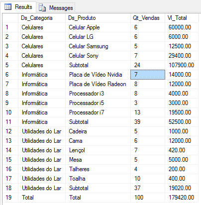
Using GROUP BY ROLLUP
A very simple and practical way to solve this problem is by using the ROLLUP() function in GROUP BY, which already creates groupings and summaries according to the columns grouped in the function.
Using this function, you will see that it creates the totalizers just below each grouping and the general totalizer in the last line of the resultset.
Example 1:
SELECT
    B.Ds_Categoria,
    B.Ds_Produto,
    COUNT(*) AS Qt_Vendas,
    SUM(B.Preco) AS Vl_Total
FROM
    #Vendas A
    JOIN #Produtos B ON A.Cd_Produto = B.Codigo
GROUP BY
    ROLLUP(B.Ds_Categoria, B.Ds_Produto)
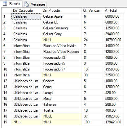
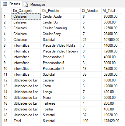
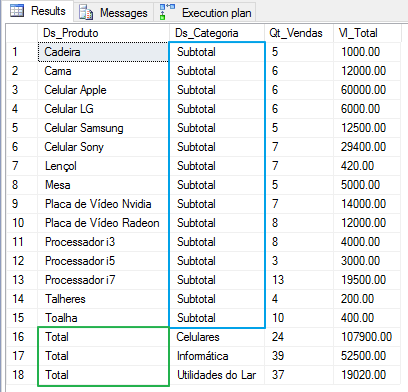
As you may have noticed, the lines containing the summaries have a NULL value in the grouped columns. In this example, the subtotal by category has the Ds_Produto column with a NULL value and in the general total, both columns have a NULL value. For our query to produce the same result as another query with UNION ALL, we simply need to treat these NULL values, as shown below:
SELECT
    ISNULL(B.Ds_Categoria, 'Total') AS Ds_Categoria,
    ISNULL(B.Ds_Produto, 'Subtotal') AS Ds_Produto,
    COUNT(*) AS Qt_Vendas,
    SUM(B.Preco) AS Vl_Total
FROM
    #Vendas A
    JOIN #Produtos B ON A.Cd_Produto = B.Codigo
GROUP BY
    ROLLUP(B.Ds_Categoria, B.Ds_Produto)
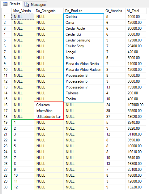
Example 2:
SELECT
    ISNULL(CONVERT(VARCHAR(10), MONTH(A.Dt_Venda)), 'Total') AS Mes_Venda,
    ISNULL(B.Ds_Categoria, 'Subtotal') AS Ds_Categoria,
    COUNT(*) AS Qt_Vendas,
    SUM(B.Preco) AS Vl_Total
FROM
    #Vendas A
    JOIN #Produtos B ON A.Cd_Produto = B.Codigo
GROUP BY
    ROLLUP(MONTH(A.Dt_Venda), B.Ds_Categoria)

Using GROUP BY CUBE
Just like the ROLLUP() function, the CUBE() function allows you to create grouped totalizers in a very practical and easy way and its syntax is the same as the ROLLUP function.
Using this function, you will see that the difference between it and ROLLUP is that the CUBE function creates totalizers for each type of grouping.
Example:
SELECT
    ISNULL(CONVERT(VARCHAR(10), MONTH(A.Dt_Venda)), 'Total') AS Mes_Venda,
    ISNULL(B.Ds_Categoria, 'Subtotal') AS Ds_Categoria,
    COUNT(*) AS Qt_Vendas,
    SUM(B.Preco) AS Vl_Total
FROM
    #Vendas A
    JOIN #Produtos B ON A.Cd_Produto = B.Codigo
GROUP BY
    CUBE(MONTH(A.Dt_Venda), B.Ds_Categoria)
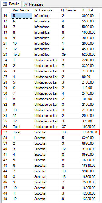
See that using the CUBE() function, I can obtain the general totalizer, the totalizer for the Month_Venda column and the totalizer for the Category column. In other words, in the CUBE function, it generates all the combination possibilities between the columns used in the function.
Using GROUP BY GROUPING SETS
Using the GROUPING SETS function in GROUP BY allows us to generate totalizers for our data using the columns inserted in the function, so that it generates different totalizers in a single query. Unlike the ROLLUP and CUBE functions, the GROUPING SETS function does not return a general totalizer.
Example 1:
SELECT
    ISNULL(B.Ds_Produto, 'Total') AS Ds_Produto,
    ISNULL(B.Ds_Categoria, 'Subtotal') AS Ds_Categoria,
    COUNT(*) AS Qt_Vendas,
    SUM(B.Preco) AS Vl_Total
FROM
    #Vendas A
    JOIN #Produtos B ON A.Cd_Produto = B.Codigo
GROUP BY
    GROUPING SETS(B.Ds_Categoria, B.Ds_Produto)
In this example, the GROUPING SETS function returns the totalizer by product and then the totalizer by category, where you would need to execute 2 queries to show this same view.
Example 2:
SELECT
    MONTH(A.Dt_Venda) AS Mes_Venda,
    B.Ds_Categoria,
    B.Ds_Produto,
    COUNT(*) AS Qt_Vendas,
    SUM(B.Preco) AS Vl_Total
FROM
    #Vendas A
    JOIN #Produtos B ON A.Cd_Produto = B.Codigo
GROUP BY
    GROUPING SETS(MONTH(A.Dt_Venda), B.Ds_Categoria, B.Ds_Produto)
In this example, the GROUPING SETS function returned the sum of the values grouped by the 3 columns that I used in the function: Sum by Sales_Month, Sum by Product and Sum by Category. To reproduce this same result, I would need to create a query with 3 queries. If there were 10 columns, the query would need 10 different queries to bring this result, which we achieved with a single query using the GROUPING SETS function.
Note: All 3 functions presented in this post accept N columns as parameters, not being limited to just 2 columns.
Performance and Performance
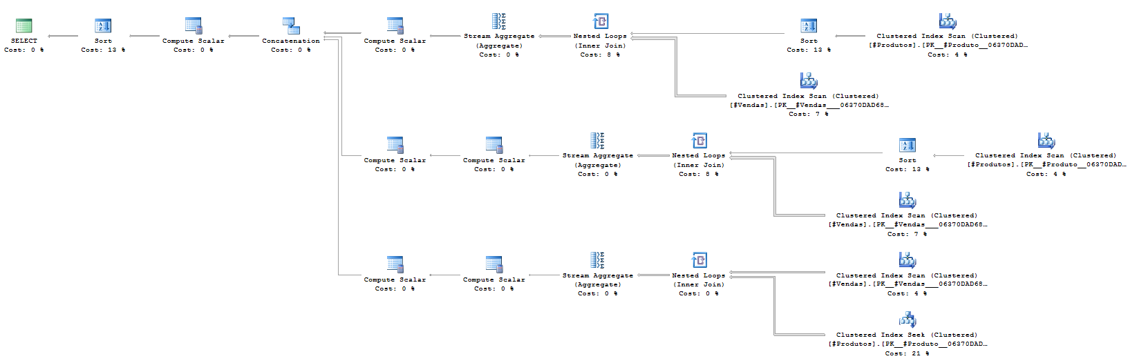
Now that we've seen how the 3 functions work and seen how practical their use is, saving many lines of code, let's analyze whether they are performant or not.
I will try to use the same query for all cases, although in some, the result (output) is different, as it really has different objectives, but just to demonstrate the cost and execution plan of each one.
UNION ALL (Example Query):
SQL Server Execution Times:
CPU time = 0 ms, elapsed time = 0 ms.
(19 row(s) affected)
Table ‘Worktable’. Scan count 0, logical reads 0, physical reads 0, read-ahead reads 0, lob logical reads 0, lob physical reads 0, lob read-ahead reads 0.
Table ‘#Products’. Scan count 2, logical reads 204, physical reads 0, read-ahead reads 0, lob logical reads 0, lob physical reads 0, lob read-ahead reads 0.
Table ‘#Sales’. Scan count 3, logical reads 64, physical reads 0, read-ahead reads 0, lob logical reads 0, lob physical reads 0, lob read-ahead reads 0.
(1 row(s) affected)
SQL Server Execution Times:
CPU time = 0 ms, elapsed time = 79 ms.
SQL Server parse and compile time:
CPU time = 0 ms, elapsed time = 0 ms.
SQL Server Execution Times:
CPU time = 0 ms, elapsed time = 0 ms.
GROUP BY ROLLUP (Query from example 1)
SQL Server parse and compile time:
CPU time = 0 ms, elapsed time = 0 ms.
SQL Server Execution Times:
CPU time = 0 ms, elapsed time = 0 ms.
SQL Server parse and compile time:
CPU time = 0 ms, elapsed time = 0 ms.
(19 row(s) affected)
Table ‘#Sales’. Scan count 1, logical reads 31, physical reads 0, read-ahead reads 0, lob logical reads 0, lob physical reads 0, lob read-ahead reads 0.
Table ‘Worktable’. Scan count 0, logical reads 0, physical reads 0, read-ahead reads 0, lob logical reads 0, lob physical reads 0, lob read-ahead reads 0.
Table ‘#Products’. Scan count 1, logical reads 2, physical reads 0, read-ahead reads 0, lob logical reads 0, lob physical reads 0, lob read-ahead reads 0.
(1 row(s) affected)
SQL Server Execution Times:
CPU time = 0 ms, elapsed time = 57 ms.
SQL Server parse and compile time:
CPU time = 0 ms, elapsed time = 0 ms.
SQL Server Execution Times:
CPU time = 0 ms, elapsed time = 0 ms.

GROUP BY CUBE (Query from example 1)
SQL Server parse and compile time:
CPU time = 0 ms, elapsed time = 0 ms.
SQL Server Execution Times:
CPU time = 0 ms, elapsed time = 0 ms.
SQL Server parse and compile time:
CPU time = 0 ms, elapsed time = 6 ms.
(49 row(s) affected)
Table ‘Worktable’. Scan count 2, logical reads 71, physical reads 0, read-ahead reads 0, lob logical reads 0, lob physical reads 0, lob read-ahead reads 0.
Table ‘#Products’. Scan count 0, logical reads 200, physical reads 0, read-ahead reads 0, lob logical reads 0, lob physical reads 0, lob read-ahead reads 0.
Table ‘#Sales’. Scan count 1, logical reads 2, physical reads 0, read-ahead reads 0, lob logical reads 0, lob physical reads 0, lob read-ahead reads 0.
(1 row(s) affected)
SQL Server Execution Times:
CPU time = 0 ms, elapsed time = 210 ms.
SQL Server parse and compile time:
CPU time = 0 ms, elapsed time = 0 ms.
SQL Server Execution Times:
CPU time = 0 ms, elapsed time = 0 ms.

GROUP BY GROUPING SETS (query from example 1)
SQL Server parse and compile time:
CPU time = 0 ms, elapsed time = 0 ms.
SQL Server Execution Times:
CPU time = 0 ms, elapsed time = 0 ms.
SQL Server parse and compile time:
CPU time = 0 ms, elapsed time = 5 ms.
(18 row(s) affected)
Table ‘Worktable’. Scan count 2, logical reads 35, physical reads 0, read-ahead reads 0, lob logical reads 0, lob physical reads 0, lob read-ahead reads 0.
Table ‘#Sales’. Scan count 1, logical reads 31, physical reads 0, read-ahead reads 0, lob logical reads 0, lob physical reads 0, lob read-ahead reads 0.
Table ‘#Products’. Scan count 1, logical reads 2, physical reads 0, read-ahead reads 0, lob logical reads 0, lob physical reads 0, lob read-ahead reads 0.
(1 row(s) affected)
SQL Server Execution Times:
CPU time = 0 ms, elapsed time = 58 ms.
SQL Server parse and compile time:
CPU time = 0 ms, elapsed time = 0 ms.
SQL Server Execution Times:
CPU time = 0 ms, elapsed time = 0 ms.

Running the 4 queries together:
SQL Sentry Plan Explorer Execution Plan

SQL Server Management Studio Execution Plan

In other words, with these tests and using this mass of data, we can say that queries performed with these functions are more performant than using subqueries with several queries to return grouped data. This does not mean that this statement will always be true, it will depend a lot on your environment and your mass of data.
I hope you liked this post.
A hug!

Comentários (0)
Carregando comentários…